Power optimum shifts earlier
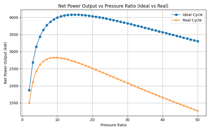
In the saved sweep, component inefficiencies and pressure losses move the modelled maximum power from PR 15 to PR 10.
THERMODYNAMICS / PYTHON / EXERGY ANALYSIS · INDEPENDENT PROJECT
A Python simulation comparing ideal-component and non-ideal Brayton gas turbine cycles. The model uses compressor and turbine efficiencies, combustor pressure loss and energy/exergy balances to examine how pressure ratio and turbine inlet temperature change predicted performance.
01 / OBJECTIVE
The aim was to quantify how departures from ideal compression and expansion affect predicted net shaft power, first-law thermal efficiency and second-law performance. Separate pressure-ratio and turbine-inlet-temperature sweeps were implemented to identify different operating points for maximum power and efficiency.
Model scope: A simplified steady-state air-standard cycle with constant specific heat and heat-capacity ratio. It is a conceptual design calculation, not an experimentally validated gas turbine or a manufacturer performance map.
02 / SYSTEM MODEL
Air temperature and pressure rise through the compressor; real outlet temperature accounts for ηc.
Working-fluid temperature increases to the specified TIT; the model applies combustor pressure loss.
The turbine delivers shaft work; actual outlet temperature depends on ηt and expansion pressure ratio.
Heat rejection is represented through the air-standard cycle idealisation.
| Input | Configuration | Meaning |
|---|---|---|
| T1 / P1 | 298.15 K / 100,000 Pa | Compressor inlet conditions |
| T3 | 1400 K baseline | Turbine inlet temperature |
| γ / Cp / R | 1.4 / 1005 J kg−1 K−1 / 287 J kg−1 K−1 | Constant air-property assumptions |
| ηc / ηt | 0.85 / 0.90 | Compressor / turbine isentropic efficiencies in real model |
| ΔPcombustor | 5% | Pressure loss is applied in both comparison models |
| T0 | 300 K | Exergy reference temperature |
The repository calls its first case the ideal cycle. More precisely, its compressor and turbine are isentropic but it retains the configured 5% combustor pressure loss. It is therefore not a completely loss-free textbook Brayton cycle.
03 / GOVERNING EQUATIONS
T2s = T1 · PR(γ−1)/γ
T2 = T1 + (T2s − T1) / ηc
T4 = T3 − ηt(T3 − T4s)
wnet = Cp[(T3 − T4) − (T2 − T1)]
ηth = wnet / [Cp(T3 − T2)]
ĖD = T0 Ṡgen
The code calculates compressor and turbine entropy changes using constant-property ideal-gas relations and applies the Gouy-Stodola relationship to calculate their exergy destruction. Its second-law efficiency uses the simplified heat-exergy approximation Qin(1 − T0/T3), not detailed fuel chemical exergy.
04 / PARAMETRIC RESULTS
The committed Results/cycle_optima_summary.csv reports these model outcomes for the saved configuration:
| Case | Optimised quantity | PR | Net power | Thermal efficiency |
|---|---|---|---|---|
| Ideal-component case | Maximum net power | 15 | 3.98 MW | 52.61% |
| Real-component case | Maximum net power | 10 | 2.73 MW | 34.99% |
| Ideal-component case | Maximum thermal efficiency* | 50 | 3.23 MW | 65.91% |
| Real-component case | Maximum thermal efficiency | 23 | 2.31 MW | 38.69% |
*The ideal-component efficiency rises to its highest recorded value at the upper sweep boundary PR = 50. This is a boundary result, not proof of a finite interior optimum.
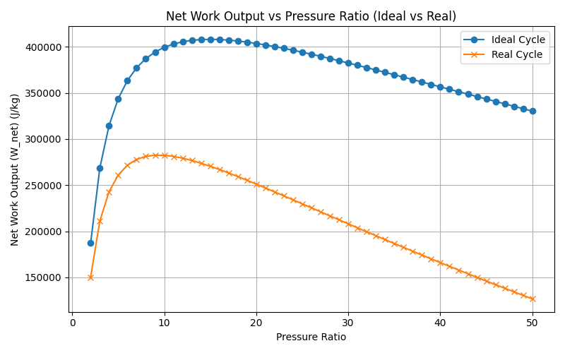
In the saved sweep, component inefficiencies and pressure losses move the modelled maximum power from PR 15 to PR 10.
Real-model thermal efficiency peaks at PR 23, where net power is lower than at PR 10. The choice depends on the design objective.
Higher pressure ratios increase compressor outlet temperature and specific compressor work, eventually eroding the power benefit of expansion.
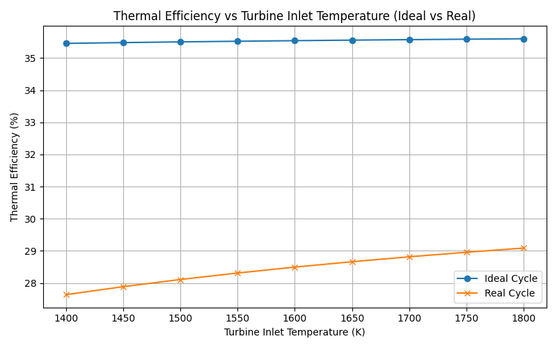
The separate TIT sweep explores 1400–1800 K. The Notion summary reports modest real-cycle efficiency gains, whereas the ideal-component efficiency is insensitive to TIT for fixed PR under the model assumptions.
05 / SECOND-LAW ANALYSIS
The simulation estimates component-level entropy generation and exergy destruction in the compressor and turbine, then compares the net work output with a simplified heat-exergy input expression.
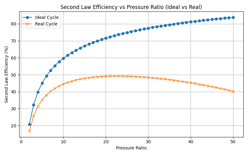
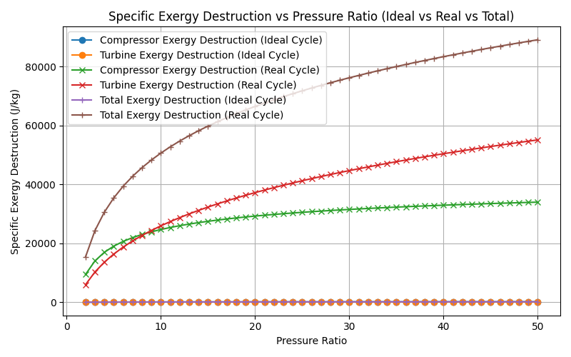
Interpretation boundary: These exergy quantities follow the repository's simplified constant-property calculations. The model does not resolve combustion chemistry, fuel exergy, heat transfer to surroundings or a complete combustor exergy balance, so the figures should not be presented as audited plant irreversibility losses.
06 / SOFTWARE
The GitHub repository separates Brayton.py (ideal/real cycle state calculations), Config.py (parameters), Sensitivity.py (sweeps), Plots.py (graph functions) and Main.py (simulation pipeline). Pandas exports the pressure-ratio runs and optimum summary to CSV.
Representative lines from the real-cycle calculation:
T2s = T1 * pressure_ratio ** ((gamma - 1) / gamma)
T2 = T1 + (T2s - T1) / compressor_efficiency

P3 = P2 * (1 - combustor_pressure_loss)
T4s = T3 * (P4 / P3) ** ((gamma - 1) / gamma)
T4 = T3 - (T3 - T4s) * turbine_efficiency

W_net = Cp * (T3 - T4) - Cp * (T2 - T1)
power_net = mass_flow_rate * W_net
The functions also reject non-physical conditions such as non-positive net work and turbine-inlet temperatures below the compressor outlet temperature.
Reproducibility note: The committed Main.py produces CSV outputs, but its individual plotting calls are currently commented out. Saved graph files remain available; to regenerate them from a fresh run, the required plotting calls must be enabled.
07 / ENGINEERING REFLECTION
The key engineering result is the trade-off between power and efficiency. Selecting pressure ratio solely for maximum ideal-cycle efficiency can miss the lower net-power optimum of the real-component model. Including imperfect components changes both the magnitude and location of the predicted performance peaks.
Next iteration: Use temperature-dependent specific heat, separate combustor exergy accounting and measured compressor/turbine maps; add structured unit tests and rerun the model against an established published benchmark. These are improvement proposals rather than completed validation.